








By Global Technology Desk
Machine learning systems that train themselves have long served as the ultimate frontier of science fiction. Today, that gap continues to narrow through systems like DeepMind’s AlphaGo and advanced large language models (LLMs). Yet, the theoretical foundations of these autonomous systems date back far further than many realize, originating in research formulated during the late 1950s.
While that timeframe may seem both a distant era in technological history and a relatively recent foundation, it marks the genesis of what the industry now classifies as Reinforcement Learning (RL).
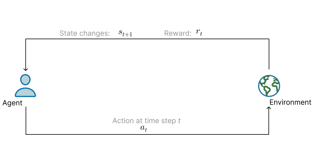
According to Google Cloud documentation, Reinforcement Learning is defined as "a type of Machine Learning where an agent learns optimal behavior through interaction with its environment. Rather than relying on explicit programming or labeled datasets, this agent learns by trial and error, receiving feedback in the form of rewards or penalties for its actions. This process mirrors how people typically learn naturally, making RL a powerful approach for creating intelligent systems capable of solving complex problems."
As artificial intelligence permeates industries ranging from robotics to natural language processing, understanding the mechanics, history, and operational challenges of RL has become essential for technologists and enterprise leaders alike.
Chronology: The Historical Evolution of Reinforcement Learning
To understand how modern artificial intelligence achieves autonomous adaptation, one must trace the field’s lineage back nearly seven decades.
1. The Roots in Optimal Control (1950s)
What modern engineers recognize as Reinforcement Learning traces its conceptual origins to the field of optimal control during the 1950s. During this period, mathematicians and engineers sought to develop methodologies and algorithms that could "learn" over time to govern dynamic systems efficiently.
A central figure in this progression was Richard Bellman, who researched methods to solve optimal control problems. Bellman’s work centered on designing controllers that followed specific rules to minimize a measure of a dynamic system over time. This foundational work birthed Dynamic Programming, paving the way for classic computational approaches such as the Bellman-Ford and Floyd-Warshall algorithms.
2. The Intersection of Control and Learning (Late 1970s–1980s)
The convergence of optimal control, dynamic programming, and machine-driven learning did not occur until the late 1970s. Paul Werbos pioneered Heuristic Dynamic Programming, which introduced neural network architectures to dynamic optimization. A decade later, Chris Watkins made a breakthrough by bridging dynamic programming methods with online learning, establishing the framework for modern value-iteration techniques.
3. Neuro-Dynamic Programming and the Modern Era (1990s–Present)
The field accelerated significantly in the mid-1990s through the contributions of Dimitri Bertsekas and John Tsitsiklis, who coined the term neuro-dynamic programming. By merging reinforcement learning with artificial neural networks, researchers laid the groundwork for deep reinforcement learning. Today, this discipline drives advanced systems like AlphaGo—which mastered the complex board game Go through self-play—as well as automated trading systems, robotic locomotion, and reinforcement learning from human feedback (RLHF) used to align LLMs.
Key Features and Core Challenges of Reinforcement Learning
Not all machine learning paradigms operate under the same operational constraints. Three primary characteristics distinguish Reinforcement Learning from supervised and unsupervised learning models.
1. Closed-Loop Architecture
RL problems are inherently closed-loop systems. The agent and the environment operate in a continuous feedback loop: the agent takes actions, and those actions directly alter the future states and inputs of the environment.
2. Absence of Explicit Instruction
Unlike supervised learning, where models train on explicitly labeled datasets containing correct answers, an RL agent receives no direct instruction manual. It must independently discover which sequence of actions yields the maximum cumulative reward.
3. Delayed Consequences
The impact of an agent’s actions may not manifest immediately. An action that appears beneficial in the short term can lead to a systemic disadvantage later—much like taking a seemingly logical shortcut through a crowded retail floor only to encounter a dead-end.
The Exploration vs. Exploitation Trade-Off
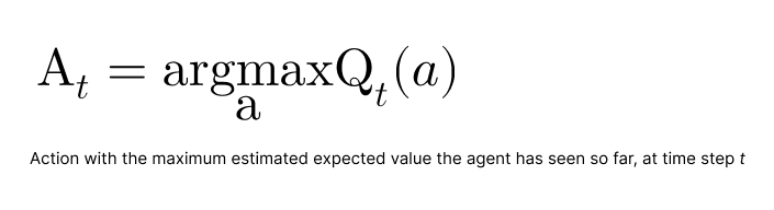
At the heart of every reinforcement learning algorithm lies a fundamental tension: the balance between exploration and exploitation.
- Exploitation involves leveraging actions that the agent has previously tested and verified as effective for generating rewards.
- Exploration requires the agent to test uncharted actions to discover potentially superior strategies that it has not yet selected.
If an agent remains purely greedy, exploiting only its immediate knowledge, it risks missing out on optimal long-term strategies. Conversely, endless exploration without exploitation prevents the system from capitalizing on proven high-value actions.
Formalizing the Reinforcement Learning Environment
To build a functioning RL algorithm, developers must orchestrate several foundational components within a systematic framework:
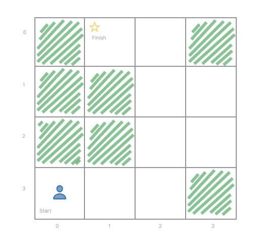
- The Agent: The autonomous entity navigating the environment and making decisions.
- The Environment: The external world or system with which the agent interacts.
- The State ($S$): The condition or configuration of the environment as observed by the agent at any given time point $t$. Every action alters this state, defining the available options for subsequent steps.
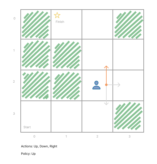
- The Policy ($pi$): The agent’s behavioral rulebook, mapping perceived states of the environment to actions. Policies can be stochastic (expressing probabilities for various actions) or deterministic (specifying a singular action per state).
- The Reward Signal ($R$): The immediate numerical feedback delivered to the agent following an action, signifying success or failure within a specific state.
- The Value Function ($V$): A long-term projection of cumulative rewards. While the reward signal evaluates immediate consequences, the value function estimates the total reward an agent can accumulate over time starting from a specific state.
- Model-Based vs. Model-Free Algorithms: Model-based architectures construct a predictive simulation of the environment to plan future actions without physical trial-and-error. In contrast, model-free algorithms rely entirely on direct interaction and experiential learning.
Supporting Data and Application: The Multi-Armed Bandit Problem
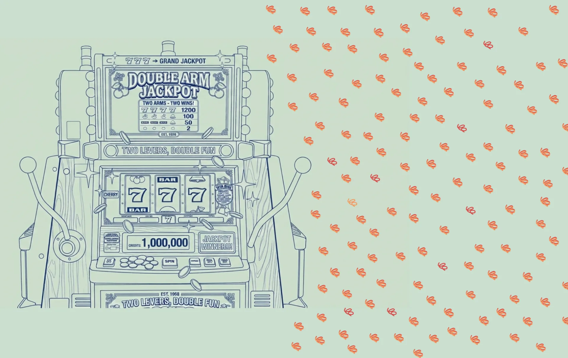
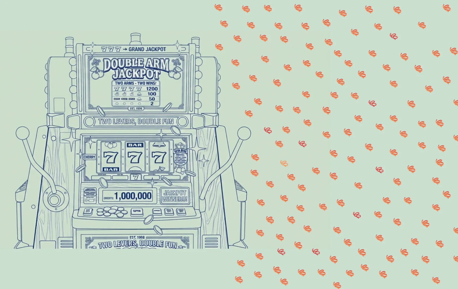
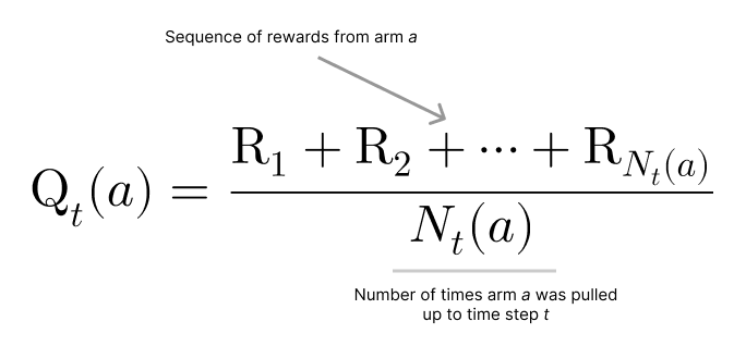
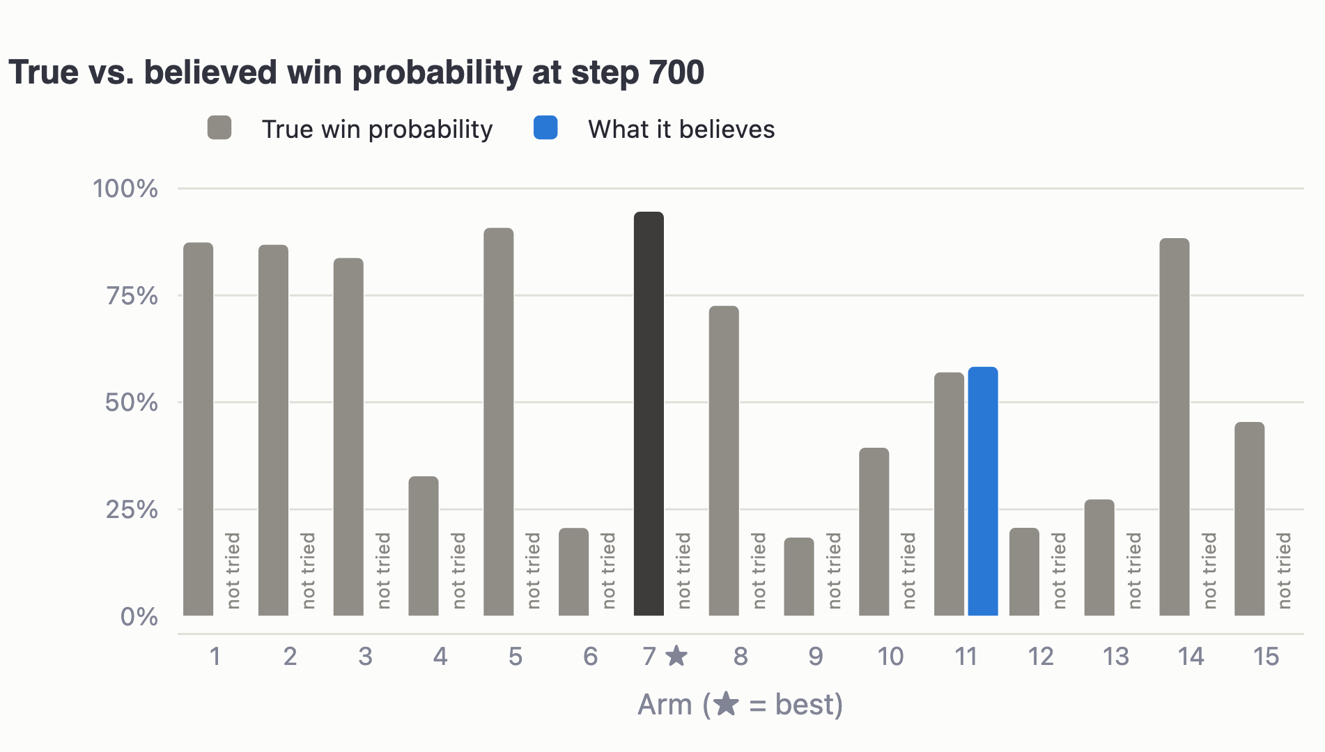
To evaluate the exploration-exploitation trade-off quantitatively, researchers frequently study the Multi-Armed Bandit (MAB) problem. Named after a traditional slot machine with multiple levers (or "arms"), the MAB problem simulates a scenario where an agent must choose among $n$ discrete actions, each yielding rewards drawn from an independent probability distribution.
Comparative Dynamics: Greedy vs. Near-Greedy (Epsilon-Greedy) Agents
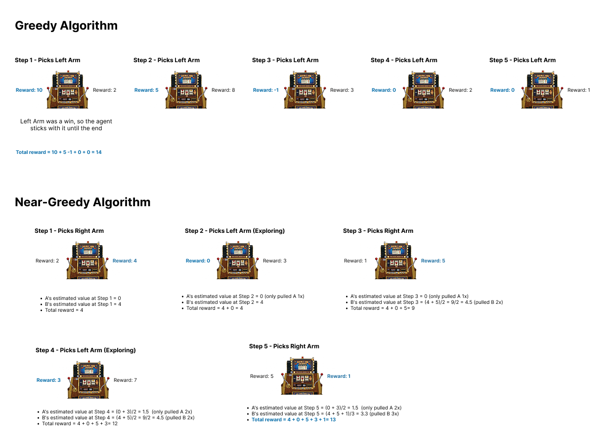
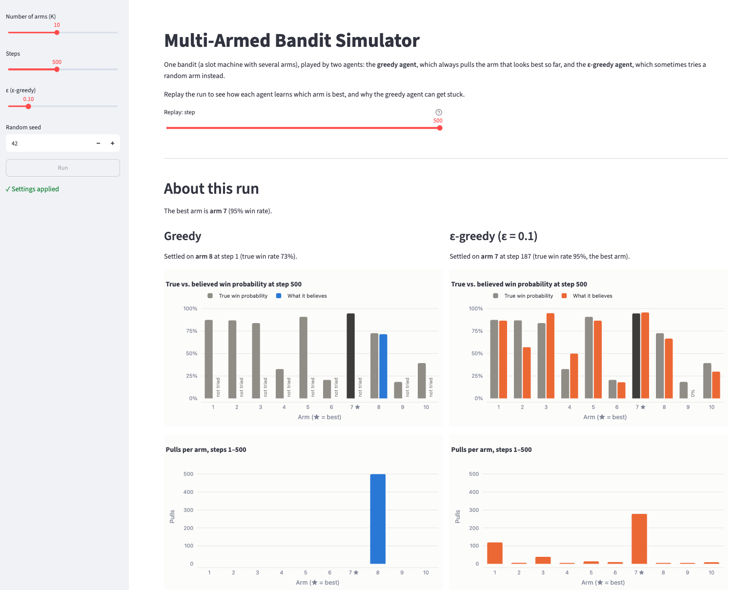
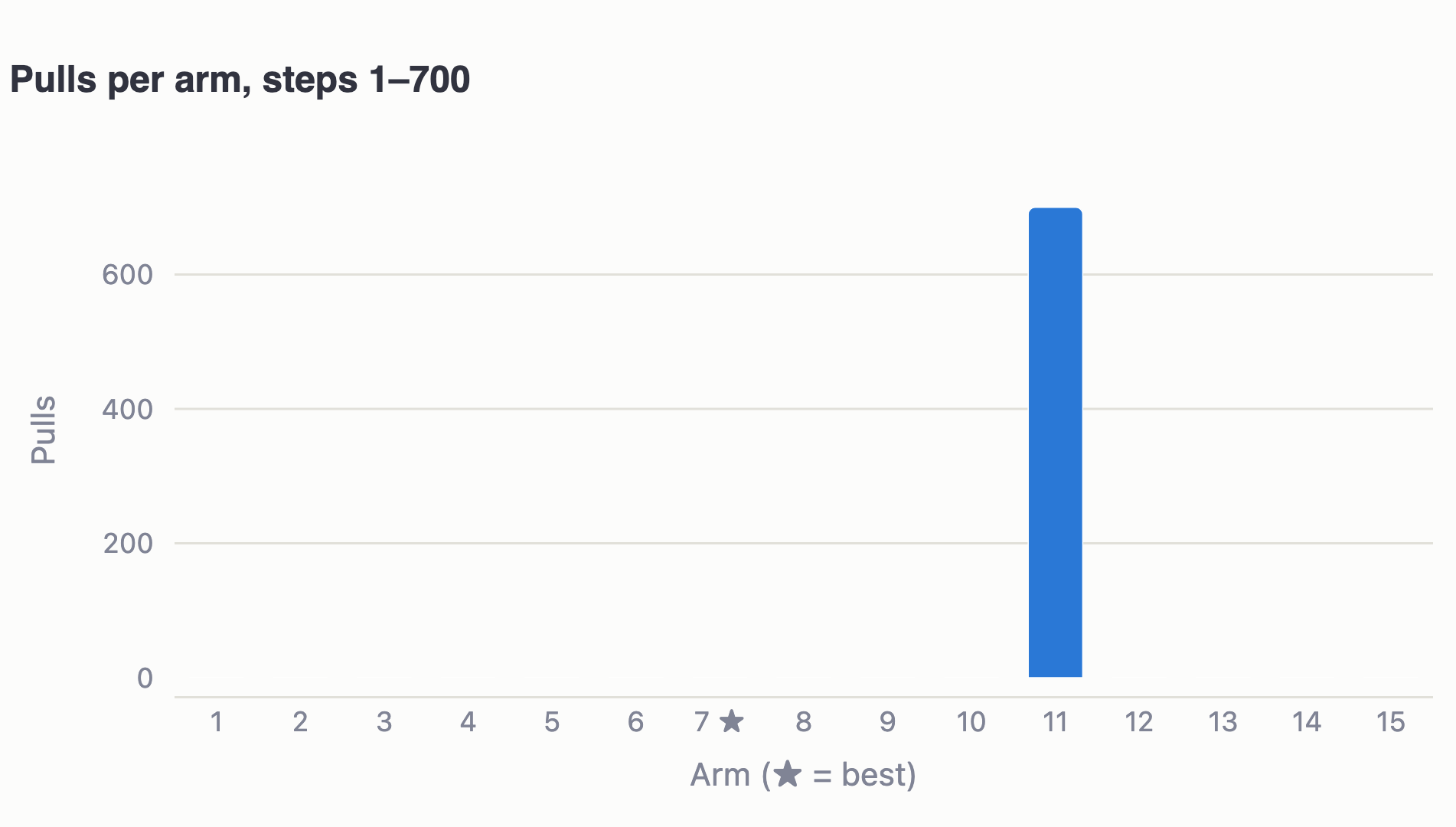
- The Greedy Agent: This agent always selects the arm with the highest estimated value based on its limited historical data. If its first pull results in a win, it assumes a 100% success rate for that arm and exploits it indefinitely, ignoring all other options.
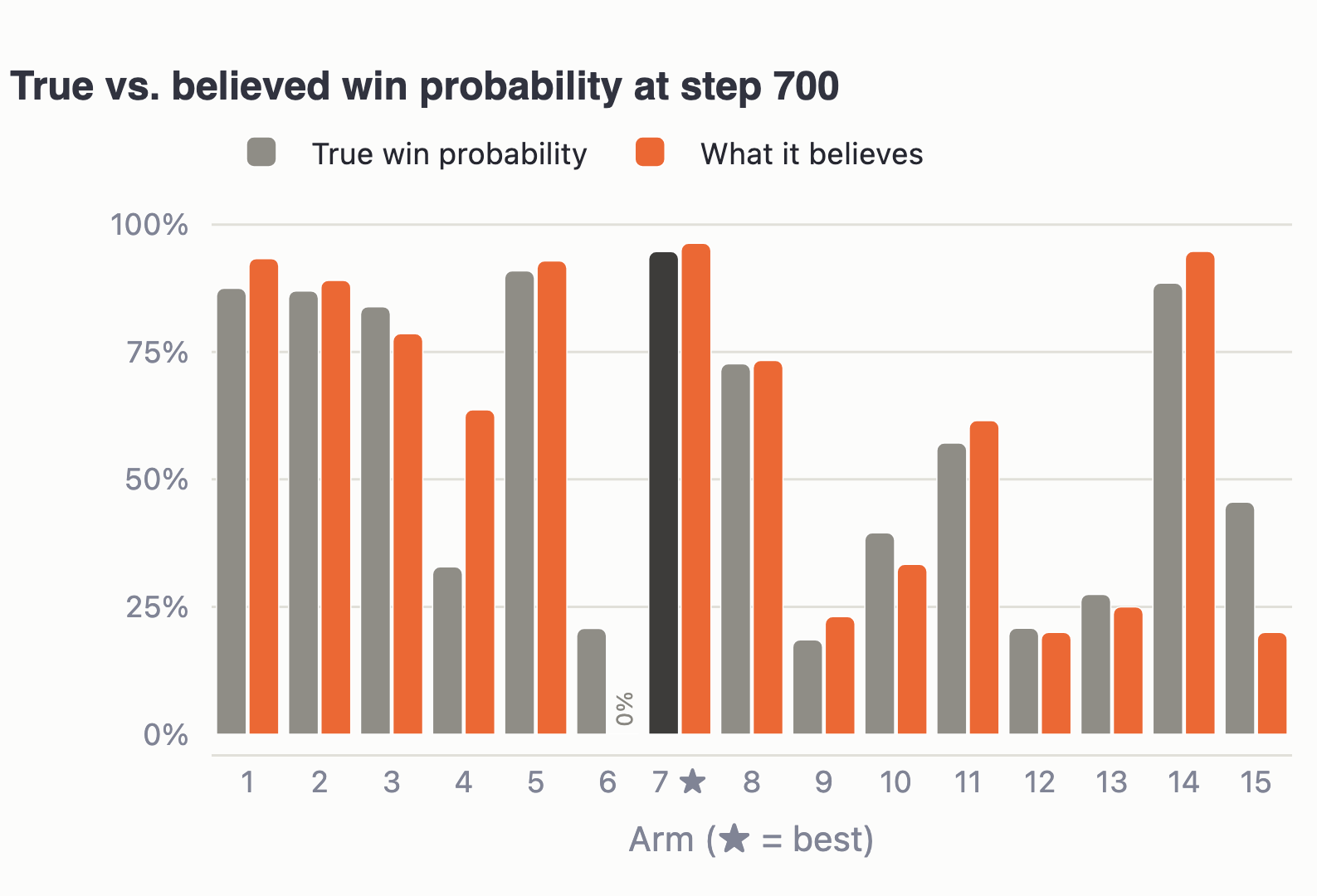
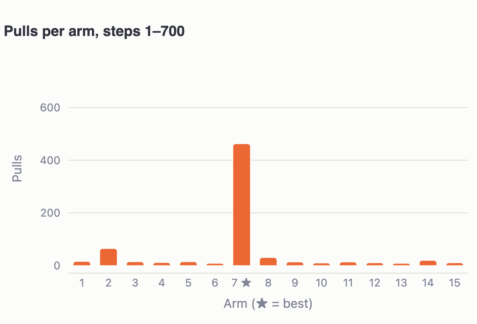
- The Near-Greedy (Epsilon-Greedy) Agent: This agent incorporates an exploration factor ($epsilon$). Most of the time, it exploits its top-performing arm, but with a predetermined probability (e.g., $epsilon = 0.1$ or $0.2$), it randomly samples alternative arms to gather new performance data.
[Agent Initialization] ---> [Environment Interaction] ---> [Reward Evaluation]
         ^                                                          |
         |------------------- (Policy Update) <---------------------|
Empirical simulations evaluating 10-arm and multi-arm bandits over hundreds of sequential steps consistently illustrate the limitations of pure greed. While a greedy agent may capture early wins based on initial luck, it frequently locks onto suboptimal options.
In contrast, a near-greedy agent absorbs short-term performance dips caused by exploration. By systematically testing alternative actions, it frequently discovers superior long-term strategies, ultimately achieving higher cumulative win rates over extended execution cycles.
Industry Implications and Official Responses
As reinforcement learning transitions from academic laboratories into enterprise infrastructure, its economic and technical implications are profound.
Tech sector leaders have increasingly integrated RL methodologies into foundational AI architectures. Leading AI developers utilize Reinforcement Learning from Human Feedback (RLHF) to ensure that generative models output helpful, honest, and harmless responses. By treating human preference ratings as reward signals, engineers can steer complex neural networks away from toxic outputs without hardcoding prohibitive content filters.
Furthermore, supply chain logistics, autonomous vehicle navigation, algorithmic financial trading, and dynamic pricing models increasingly rely on multi-armed bandit frameworks and model-free RL algorithms to optimize real-time decision-making in volatile environments.
Industry experts emphasize that as compute power scales, the adoption of model-based reinforcement learning will accelerate, enabling systems to simulate complex real-world physical and financial scenarios safely before deploying actions in live environments.
Conclusion
Reinforcement learning bridges the gap between passive data consumption and active autonomous intelligence. From its mathematical roots in 1950s optimal control theory to its modern manifestation in neural network fine-tuning and autonomous robotics, RL remains an indispensable pillar of artificial intelligence research.
By mastering the delicate balance between exploitation and exploration, reinforcement learning algorithms continue to push the boundaries of what machines can achieve independently, promising an increasingly adaptive technological future.