










By [Author Name/Staff Science Writer]
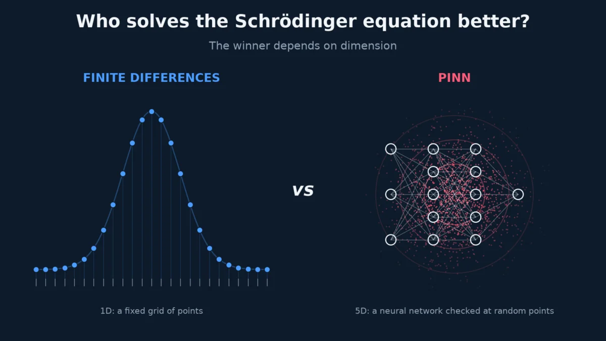
In the contemporary landscape of artificial intelligence and scientific computing, few buzzwords carry as much weight as Physics-Informed Neural Networks, or PINNs. Promoted as a paradigm-shifting alternative to traditional numerical solvers, PINNs promise an elegant shortcut: rather than discretizing space into millions of individual grid points or constructing complex meshes, researchers simply encode the governing physical equations directly into a neural network’s loss function. From there, the network learns to approximate the answer smoothly and continuously.
Yet, for all their conceptual appeal and ubiquity in modern literature, a nagging question persists among veteran computational physicists: Better than what?
Too often, flashy machine-learning demonstrations in academic journals omit comparisons against robust, classical numerical methods. A landmark 2024 study published in Nature Machine Intelligence underscored this concern, revealing that weak baselines are troublingly common in scientific machine learning, inadvertently inflating the perceived utility of AI-driven solvers.
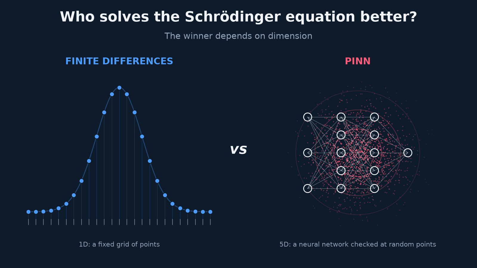
To pierce through the marketing hype and separate genuine technological leaps from computational illusions, one computational physicist decided to run a rigorous, head-to-head benchmarking test. By pitting a PINN against a classical finite-difference solver on a well-understood quantum mechanics problem, the results reveal a nuanced, dimension-dependent reality that every computational scientist needs to understand.
Main Facts: The Quantum Harmonic Oscillator Benchmark
To measure accuracy without guesswork, the experiment required a physical system with an exact, analytically known solution. The choice fell upon the quantum harmonic oscillator—essentially the quantum-mechanical equivalent of a marble rolling inside a parabolic bowl.
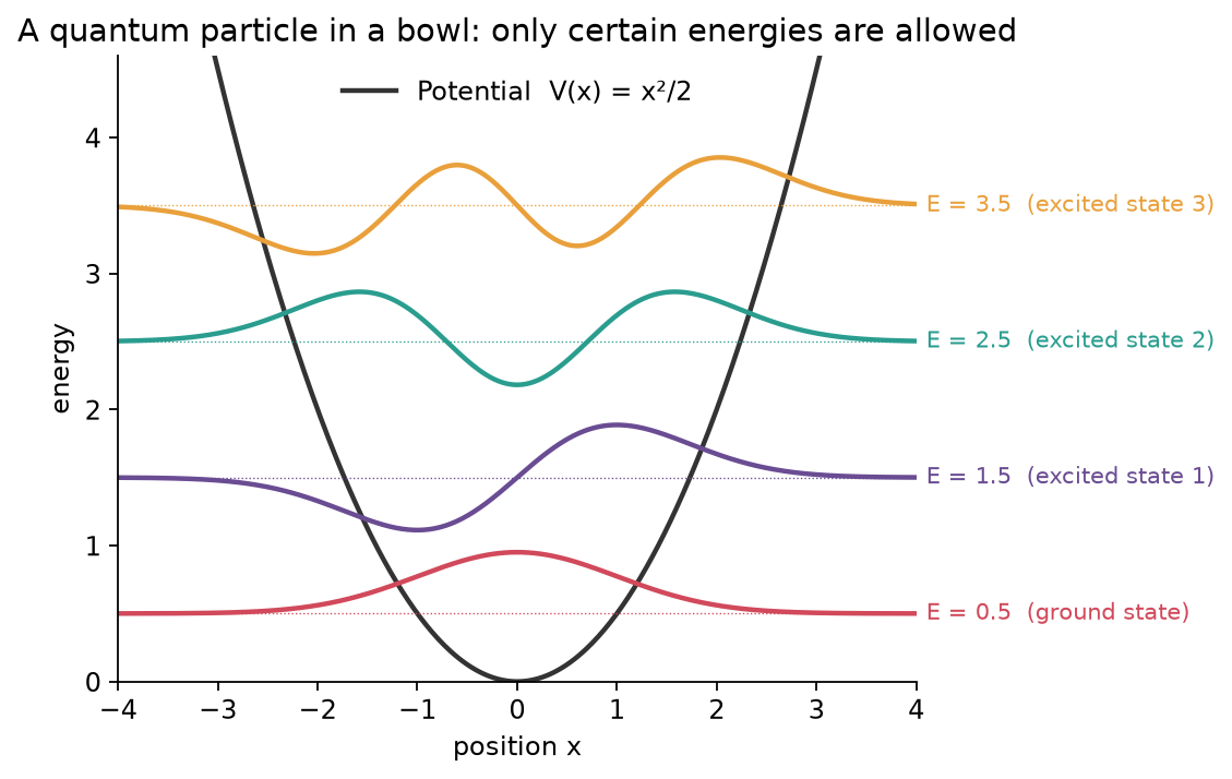
In classical mechanics, a marble can settle at any continuous energy level. A quantum particle, however, is restricted to discrete "rungs" on an energy ladder. Each rung corresponds to a specific shape known as a wavefunction ($psi(x)$), the square of which dictates the probability distribution of finding the particle at any given point in space.
The governing rule for this system is the time-independent Schrödinger equation. Using natural units ($hbar = m = omega = 1$), the Hamiltonian ($H$) operator acts as a mathematical recipe that takes a trial wavefunction shape, transforms it, and returns a new shape. The allowed physical states are the special "eigenstates" that return unchanged, save for multiplication by a numerical energy eigenvalue ($E$).
The computational challenge is twofold: the solver must determine both the energy ($E$) and the corresponding wavefunction ($psi$) simultaneously.
The Two Contenders
The experiment compared two fundamentally different approaches to finding this elusive curve:
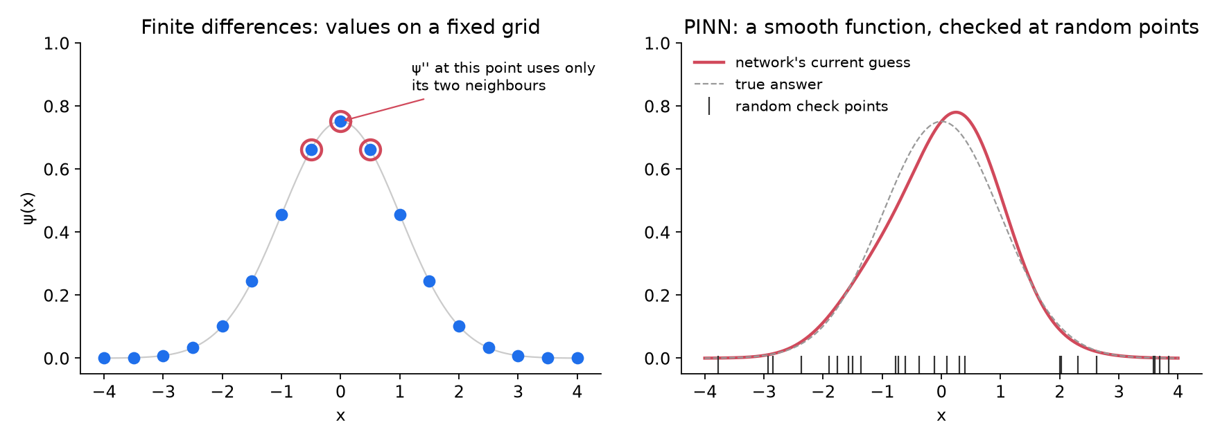
- The Finite Differences Method: A classical workhorse. This approach lays down a static grid of $N$ points along each axis, replacing continuous derivatives with algebraic formulas that reference neighboring points. The Schrödinger equation thus transforms into a massive, sparse matrix, allowing standard linear algebra packages (like SciPy) to extract the lowest eigenvalue directly. It requires zero training; the only variable is grid density ($N$).
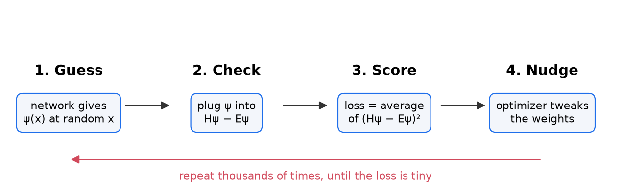
- The Physics-Informed Neural Network (PINN): In this paradigm, a small multi-layer neural network is the wavefunction. Fed a spatial coordinate $x$, it outputs a numerical value $psi(x)$. Starting from random weights, the network is trained using the governing equation itself as a teacher—requiring no pre-labeled training data. The loss function compels the network to satisfy the eigenvalue relation across random spatial points, while computing the energy dynamically via the Rayleigh quotient to ensure the energy consistently matches the current wavefunction.
Chronology: From 1D Simplicity to High-Dimensional Realities
The testing protocol was executed in two distinct phases: first in a simple one-dimensional space, and subsequently scaled up to a five-dimensional domain to test the limits of both architectures.
Phase 1: The One-Dimensional Trial
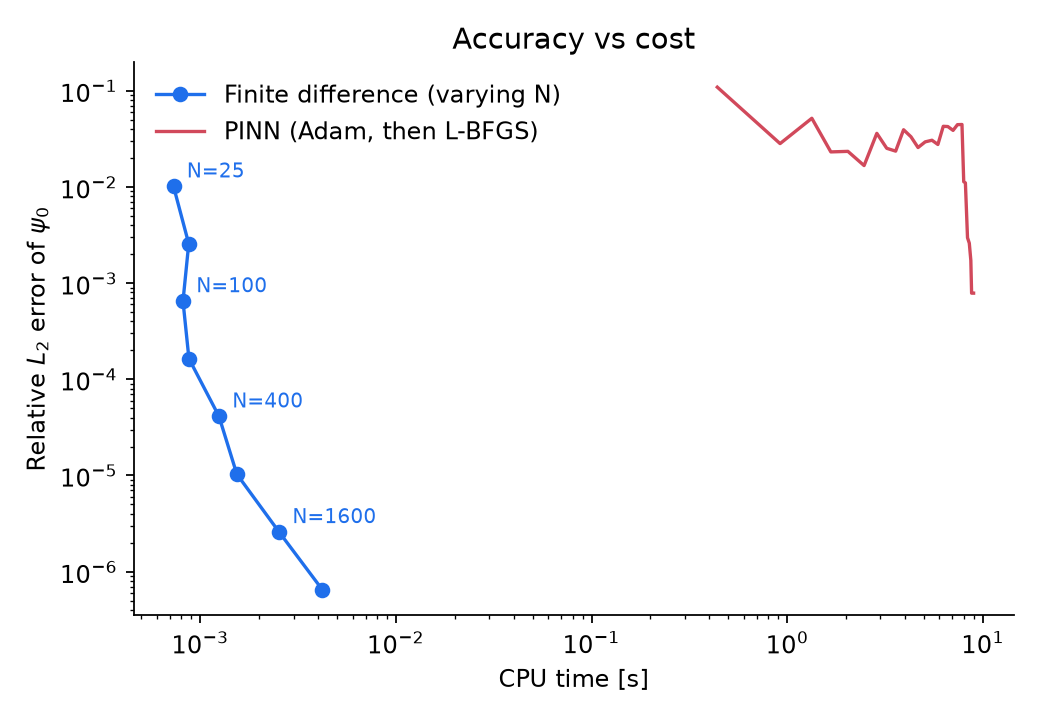
In the 1D test, both methodologies successfully identified the correct ground state. However, the computational cost diverged dramatically.
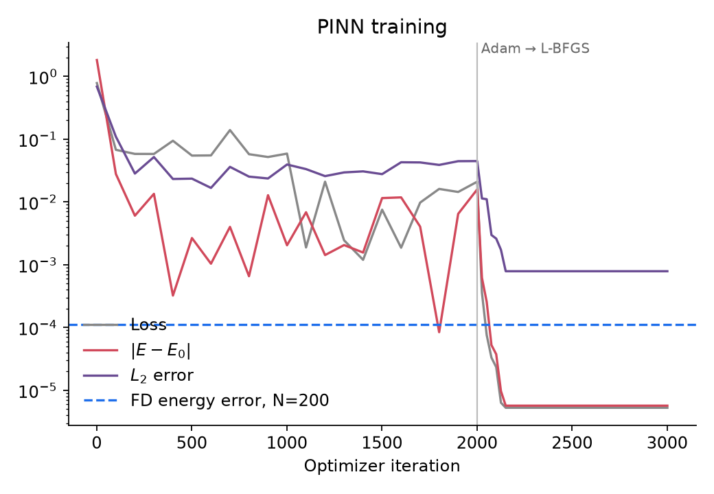
While finite difference methods achieved high accuracy in under a millisecond, the PINN struggled initially. Without intervention, training a PINN using standard first-order optimizers like Adam caused the error to stall at a few percent, trapped in a noisy plateau.
The breakthrough came via a two-stage training strategy: using Adam to coarsely rough out the shape of the wavefunction, followed by L-BFGS—a quasi-Newton optimization method—to polish the result. Within a few hundred iterations of L-BFGS, the PINN error plummeted by a factor of fifty.
- The Catch: Despite L-BFGS rescuing the PINN, the classical finite-difference method won the 1D race by a factor of roughly 10,000. For low-dimensional problems, building, training, and optimizing a neural network is an unnecessary overcomplication.
Phase 2: Scaling to Five Dimensions
Next, the complexity was increased to five dimensions ($5textD$). While five dimensions sounds like science fiction, it is a routine threshold in computational physics: tracking even two interacting particles in a three-dimensional space requires six spatial coordinates.
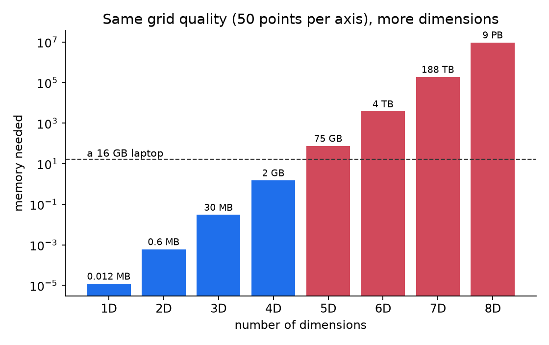
This is where the classical grid method encounters its nemesis: the curse of dimensionality.
If a grid requires $N$ points per axis, an $n$-dimensional grid requires $N^n$ total points. At a modest $N = 16$ per axis, a 5D grid demands one million unknowns and roughly 0.3 gigabytes of memory. Pushing that grid density to match the accuracy of advanced solvers would require billions of unknowns and terabytes of RAM—effectively crashing standard laptop hardware.
Conversely, a PINN does not rely on a rigid grid. By sampling random points, its memory footprint scales much more gracefully.
Supporting Data and Technical Hurdles
The 5D PINN did not succeed out of the box; it required careful structural engineering to overcome common machine learning failure points:
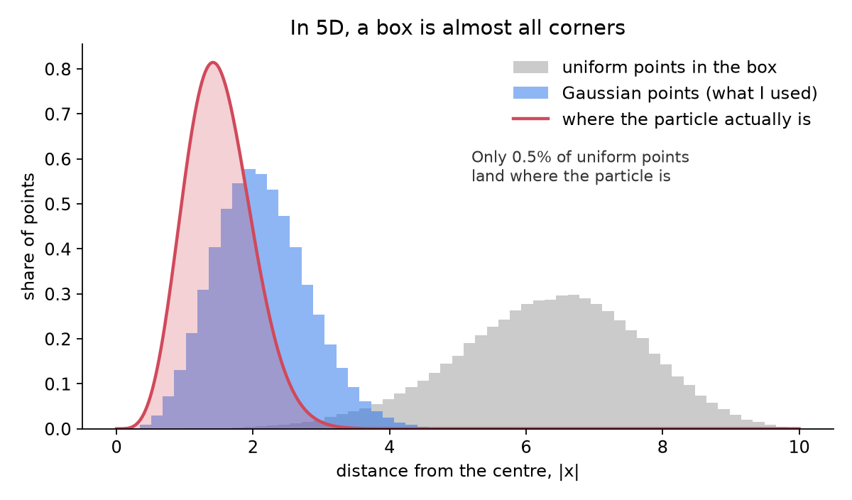
- Sampling Bias: Uniform random sampling in high dimensions causes points to pile up uselessly in distant spatial corners, with less than 0.5% landing where the physical particle actually resides. Shifting to Gaussian sampling resolved this.
- Symmetry and Nodes: Ground states cannot possess nodes (points where the wavefunction crosses zero and changes sign). To prevent the network from accidentally converging on excited states, the wavefunction was parameterized as $psi(x) = f(x) exp(-textnetwork(x))$, where a boundary factor $f(x)$ forces the wavefunction to vanish at the simulation walls, and the exponential function guarantees it remains strictly positive everywhere.
| Method | Unknowns / Parameters | Memory Footprint | CPU Time | Energy Error ($E$) | L₂ Wavefunction Error |
|---|---|---|---|---|---|
| Finite Difference ($N = 16$) | 1.0 million | 0.3 GB | 3.7 seconds | $5.5 times 10^-2$ | $3.8 times 10^-2$ |
| Finite Difference ($N approx 86$, Extrapolated) | 4.7 billion | ~1,400 GB | N/A | N/A | $sim 1.1 times 10^-3$ |
| PINN (Adam + L-BFGS) | ~9,000 weights | < 0.1 GB | 89 seconds | $6.3 times 10^-5$ | $1.1 times 10^-3$ |
As the comparative data demonstrates, the performance narrative completely inverts in higher dimensions. While the grid method hit a computational brick wall at one million unknowns (yielding a 4% error), the PINN achieved an exceptional 0.1% error within 89 seconds, compressing the entire solution into a lean network of roughly 9,000 weights.
Official Responses and Expert Perspectives
The findings echo growing sentiment within the computational mathematics community regarding the appropriate deployment of AI solvers.
Experts note that the 5D harmonic oscillator chosen for this test is mathematically "separable"—meaning it can be mathematically split into five independent 1D problems. A specialized classical solver utilizing separation of variables or tensor decomposition methods would effortlessly solve it in milliseconds. Therefore, the PINN demonstrated superiority specifically over a generic grid solver, rather than bypassing all classical mathematical ingenuity.
However, computational chemists and physicists emphasize that real-world systems—such as interacting multi-electron atoms or molecules with complex coupled potentials—are decidedly not separable. In those domains, classical tricks fail, leaving researchers constrained by exponential scaling. This exact limitation is why advanced neural-network wavefunction architectures, such as FermiNet and PauliNet, have rapidly evolved into indispensable tools for modern quantum chemistry.
Implications for the Future of Scientific Computing
The takeaway for researchers, engineers, and data scientists is clear: context is everything.
- Low Dimensions Favor Classics: In low-dimensional regimes (1D to 3D), traditional numerical methods like finite differences or finite elements remain exceptionally fast, predictable, and superior. Training a neural network for these problems is often an inefficient detour.
- High Dimensions Demand Alternatives: As systems scale into higher dimensions where tensor-product grids experience memory exhaustion, mesh-free machine learning architectures offer a viable path forward.
- Skepticism is Essential: The scientific community must maintain rigorous benchmarking standards. When evaluating new physics-informed machine learning papers, researchers should consistently ask: How would a well-tuned classical baseline perform using the exact same computational budget?
Ultimately, Physics-Informed Neural Networks are not a universal silver bullet that renders decades of numerical analysis obsolete. Rather, they are a specialized, highly potent weapon in a broader computational arsenal—one whose true power is unlocked only when applied to the high-dimensional frontiers where traditional grids fear to tread.
For researchers wishing to replicate these findings or test custom potentials, the complete Python benchmarking scripts and documentation are publicly available on GitHub at github.com/Samit1424/pinn-vs-fd-schrodinger.