Main Facts: The Structural Flaw of Traditional Forecasting

For decades, the standard approach to time series forecasting has relied on a fundamental, yet deeply flawed, mathematical assumption: that uncertainty can be neatly packaged into a single, symmetric bell curve. Whether training models using Mean Squared Error (MSE) or implementing standard Gaussian negative log-likelihood (NLL) loss, forecasters implicitly assume a world where the future is distributed normally around a single predicted mean.

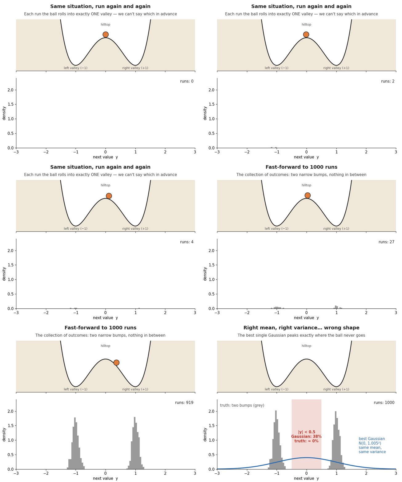
However, real-world systems rarely behave so predictably. Many processes are characterized by branching futures—such as a system teetering on a threshold where it can sharply diverge in one of two opposite directions. In these scenarios, a traditional Gaussian model yields a catastrophic failure mode: it accurately calculates the mean and variance, yet places its highest probability precisely where the system never actually goes.

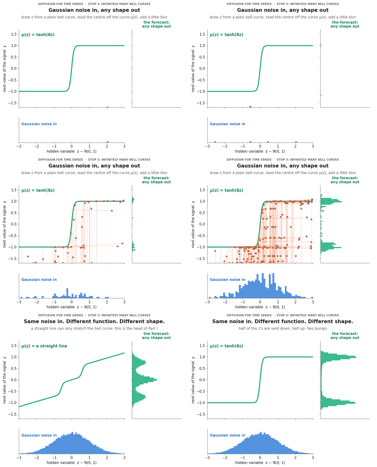
To overcome this limitation, advanced machine learning practitioners are turning to a paradigm borrowed from generative computer vision: diffusion models. Rather than mapping uncertainty as a single bell curve, time series diffusion models construct an infinite mixture of distributions, allowing forecasters to capture complex, multimodal shapes without abandoning the computational stability of standard MSE loss during training.

Chronology: The Evolution of Probabilistic Forecasting

The journey toward robust probabilistic forecasting has evolved across a distinct three-part progression, moving systematically from the size of uncertainty to its propagation, and finally to its shape.

Part I: Fixing the Size of Uncertainty

The first breakthrough stemmed from the observation that two forecasting models can yield identical MSE values while exhibiting vastly different risk profiles. Training with MSE assumes a Gaussian distribution with a fixed width. The initial fix introduced a second output head dedicated to predicting variance, optimized via Gaussian negative log-likelihood. While this solved the static sizing of uncertainty, it immediately exposed a secondary vulnerability.

Part II: Managing Uncertainty Across Time

When researchers attempted to scale the two-head model beyond a single step ahead, the system quietly broke down. Feeding predicted mean values back into the model in an autoregressive rollout created a compounding delusion—pretending every prior prediction was infallible. The repair required substituting deterministic means with sampled trajectories and executing numerous rollouts to preserve error propagation.

Part III: Capturing the Shape of Uncertainty

Even with variance heads and sampled rollouts, forecasters remained constrained by the symmetry of a single bell curve. This final evolution shifts the methodology from a single bell curve to a mixture of $K$ curves, then to a continuous infinite mixture, and ultimately to a diffusion model. By embedding a diffusion head into the autoregressive rollout framework established in earlier phases, models can now accurately forecast signals that jump, switch states, or branch into entirely different regimes.

Supporting Data: Evaluating the Double-Well Experiment

To rigorously test the efficacy of diffusion-based time series forecasting, researchers simulated a physical system: a ball rolling in a landscape with two potential energy wells ($x = -1$ and $x = +1$) separated by a fragile central barrier ($x = 0$). Driven by environmental noise, the system occasionally crosses the threshold, creating a bimodal distribution of future states.

When comparing a traditional Gaussian head against a diffusion head on contexts ending near the barrier, the limitations of the former become starkly apparent:

• True Physics (Target Distribution): Exhibits two distinct peaks in the wells, with only 6.6% of outcomes lingering on the central barrier.
• Gaussian Head: Generates a broad, single-peaked distribution centered squarely on the barrier, resulting in 12.8% of forecasts landing in a region the system practically never visits.
• Diffusion Head: Successfully recovers the bimodal shape, recording a barrier share of just 5.8%, closely mirroring the true physical system.

Interestingly, broad distributional metrics such as the Continuous Ranked Probability Score (CRPS) showed the Gaussian head and diffusion head performing nearly identically (0.494 vs. 0.493). This statistical blind spot underscores a vital warning for data scientists: sophisticated summary scores can completely mask critical failures in geometric shape.

Official Responses and Theoretical Reconciliation

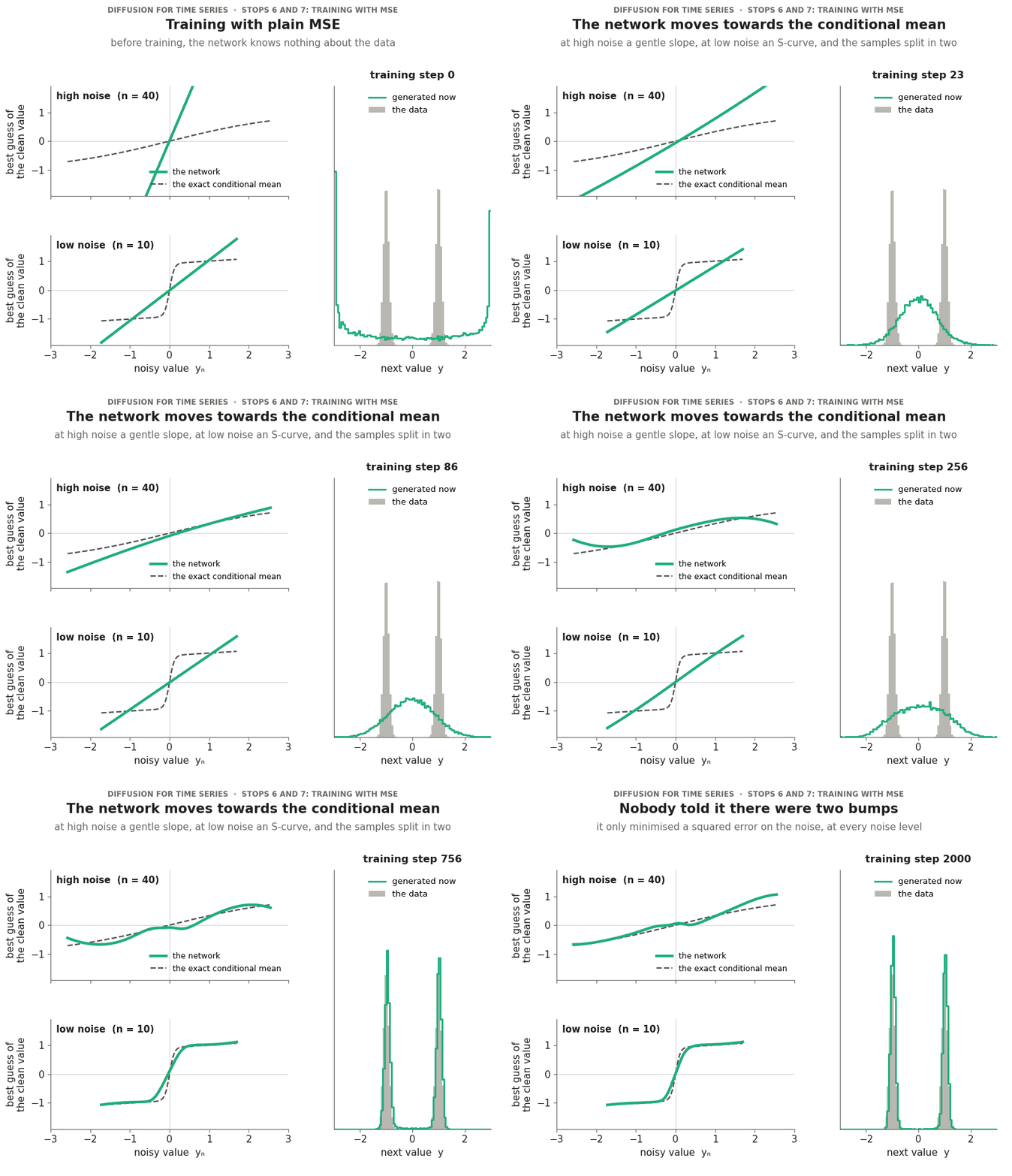
One of the most counterintuitive aspects of adopting diffusion models for time series is their reliance on plain Mean Squared Error (MSE) during training. Critics often question how an algorithm known for producing flat, regression-to-the-mean predictions can suddenly capture complex, multimodal futures.

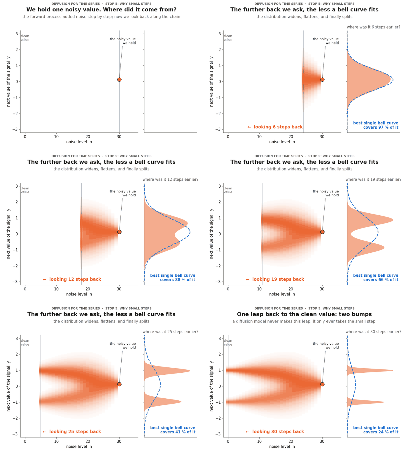
The reconciliation lies in the framing of the objective function. A traditional MSE model is asked a single, static question: "What is the future on average?" In contrast, a diffusion model is trained via a family of denoising tasks across $N$ distinct noise levels.

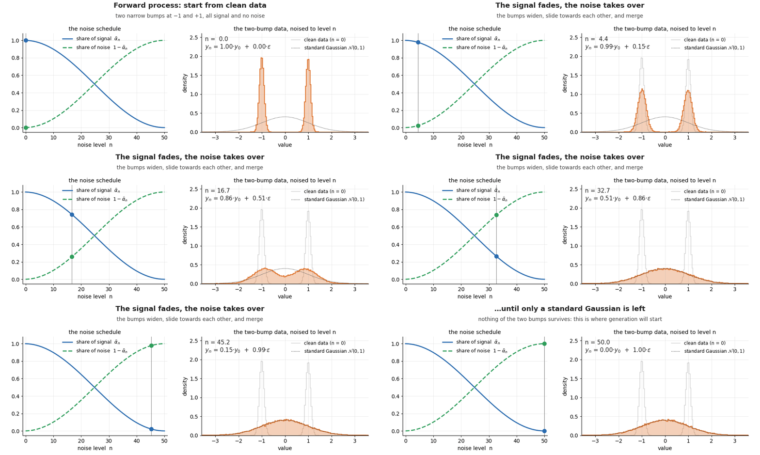
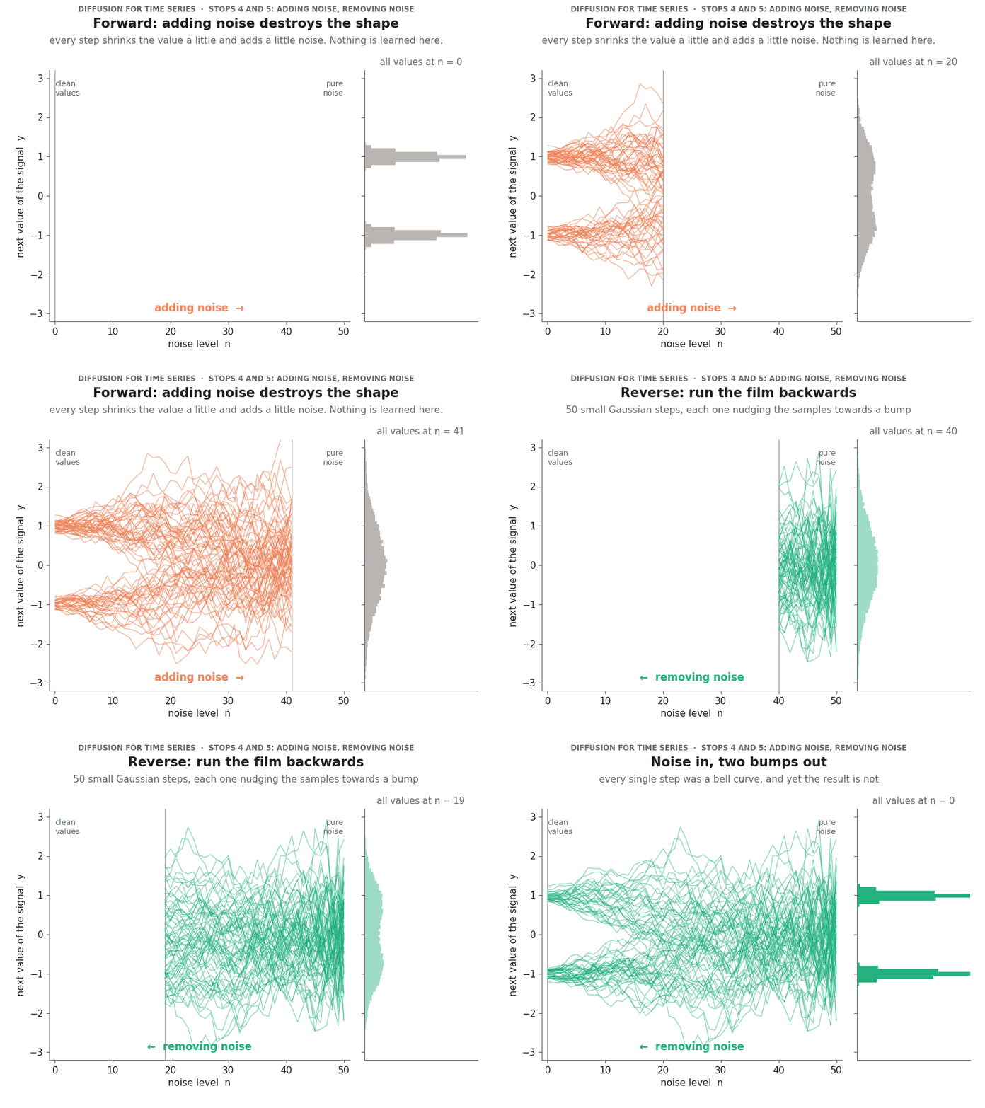
By systematically corrupting training data with a known forward noising process—governed by a variance-preserving cosine schedule—and training a neural network to predict the added noise via MSE, the model learns the conditional mean of the noise at every conceivable noise level. When these steps are reversed iteratively during inference, this tower of conditional means reconstructs an infinite mixture of Gaussian components, breathing complex shape back into the forecast.

Implications for Applied Machine Learning

The integration of diffusion models into time series forecasting carries profound implications across industries reliant on high-stakes sequential predictions, such as energy grid management, financial risk modeling, and industrial IoT monitoring.

1. The End of "Averaging Fallacies"

In systems governed by threshold effects—where missing a critical transition means the difference between system stability and catastrophic failure—relying on expected values is dangerous. Diffusion forecasting ensures that decision-makers are presented with realistic, branching trajectories rather than smoothed-out averages that exist only on paper.

2. Computational Trade-Offs

While diffusion heads dramatically improve structural fidelity, they introduce non-trivial computational overhead. Generating a single forecast requires running an iterative reverse sampling loop (e.g., 50 successive network evaluations), which is orders of magnitude slower than a single forward pass of a deterministic model. Practitioners must weigh the necessity of distributional accuracy against latency constraints in production environments.

3. A Shift in Evaluation Standards

As demonstrated by the divergence between CRPS scores and actual barrier-crossing behavior, automated evaluation metrics must evolve. Future validation frameworks must incorporate shape-aware diagnostics and visual rollout inspections to ensure that models are not merely hitting statistical benchmarks while generating physically impossible futures.