In the landscape of artificial intelligence, understanding how neural networks process information is akin to understanding the building blocks of modern computation. For many, the journey begins with a foundational concept from elementary algebra: the straight-line equation, $y = ax + b$.

While linear equations provide an intuitive entry point—a topic explored extensively in previous primers on linear neural models—they harbor a fundamental limitation. Real-world phenomena rarely conform to a single, constant rate of change. From economic shifts to human learning patterns, data is inherently messy, complex, and non-linear.

To bridge the gap between simple linear approximation and the complex predictive capabilities of modern deep learning, neural networks rely on a crucial mathematical mechanism: non-linearity. By utilizing functions such as piecewise linear curves, Rectified Linear Units (ReLU), and sigmoid curves, artificial neural networks can capture intricate patterns that defy straight-line descriptions.

---

1. Main Facts: The Limitation of Linearity and the Power of Activation Functions

At the heart of any neural network are interconnected nodes, or "neurons," which take inputs, apply weights and biases, and pass the result through an activation function.

• The Linear Constraint: A standard linear equation ($y = ax + b$) assumes that a proportional change in the input ($x$) results in a proportional, constant change in the output ($y$). The slope ($a$) and the y-intercept ($b$) remain fixed across all values.
• The Reality of Data: Real-world data exhibits changing behaviors. Variables may remain dormant up to a threshold, surge rapidly under specific conditions, and eventually plateau.
• The Role of Non-Linearity: Non-linear activation functions allow neurons to alter their behavior depending on the range of input values. This capacity transforms a collection of linear operations into a powerful, flexible computational engine capable of modeling multi-layered, complex relationships.

---

2. Chronology: From Linear Assumptions to Adaptive Networks

To understand how neural networks evolved to handle complexity, it is helpful to follow an educational case study popularized by educators like Ms. Poly, a mathematics teacher seeking to optimize her students’ study habits.

Phase I: The Straight-Line Hypothesis

Initially, Ms. Poly sought to predict final exam scores based entirely on a single metric: the number of hours a student studied per week. Assuming a direct proportionality, she deployed a standard linear formula ($y = ax + b$), where $y$ represented the marks scored, $x$ the study hours, $a$ the marginal gain per hour, and $b$ the baseline score achievable without studying.

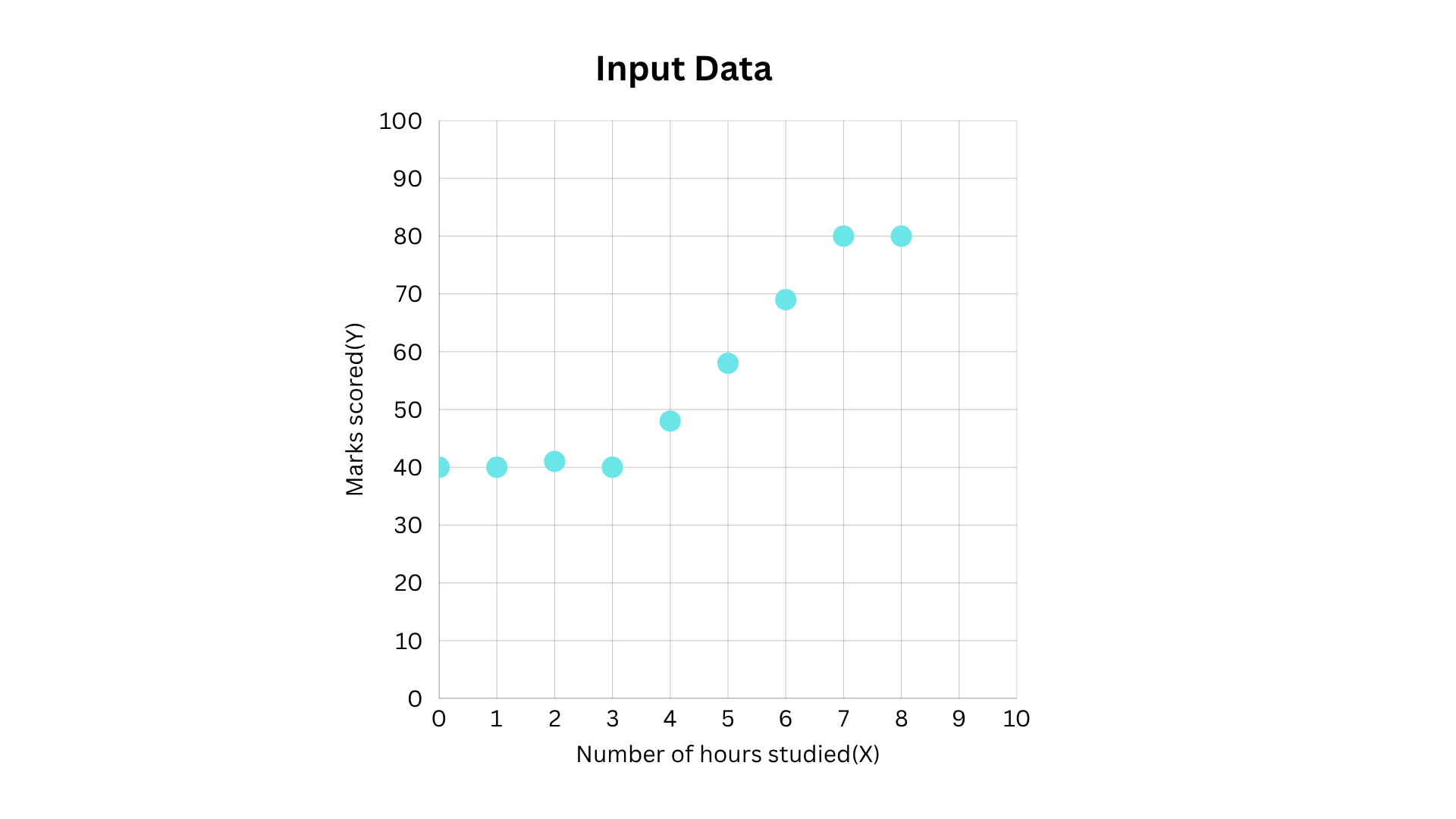
However, when she interviewed her students after a quarterly exam and plotted their weekly hours against their actual scores, the hypothesis fell apart.

Number of Hours Studied	Marks Scored
0	40
1	40
2	41
3	40
4	48
5	58
6	69
7	80
8	80

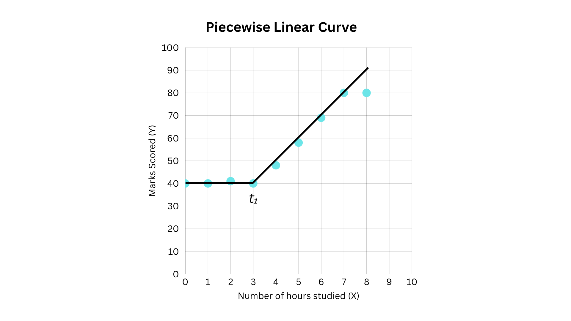
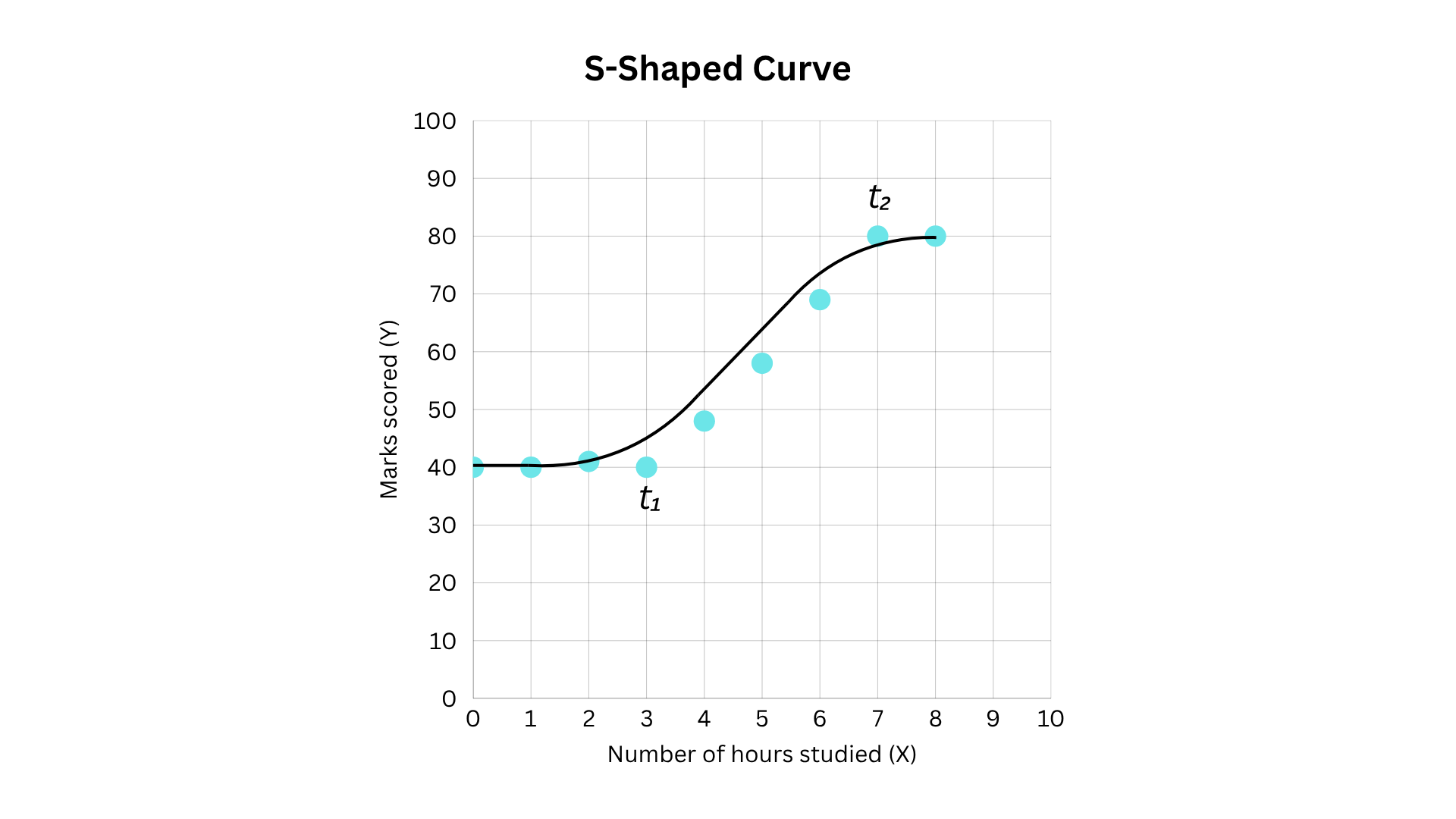
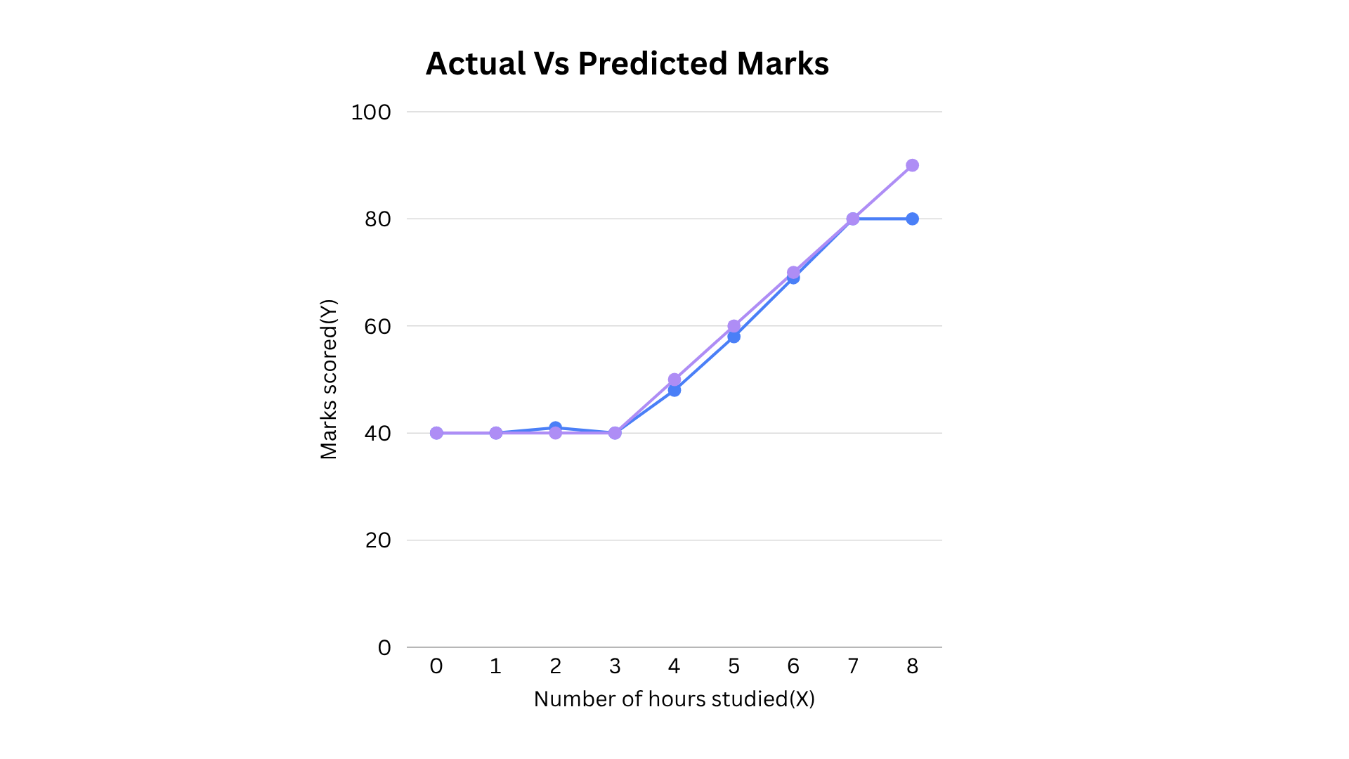
The empirical data exposed the core flaw: low study hours yielded little to no improvement; intermediate hours produced a sharp, steep increase in grades; and high study hours resulted in a performance ceiling where additional effort yielded diminishing returns. A single straight line could not possibly reconcile these three distinct behavioral phases.

Phase II: The Piecewise Linear Transition

Recognizing that the dataset required segmented rules, Ms. Poly divided the graph into three operational zones:

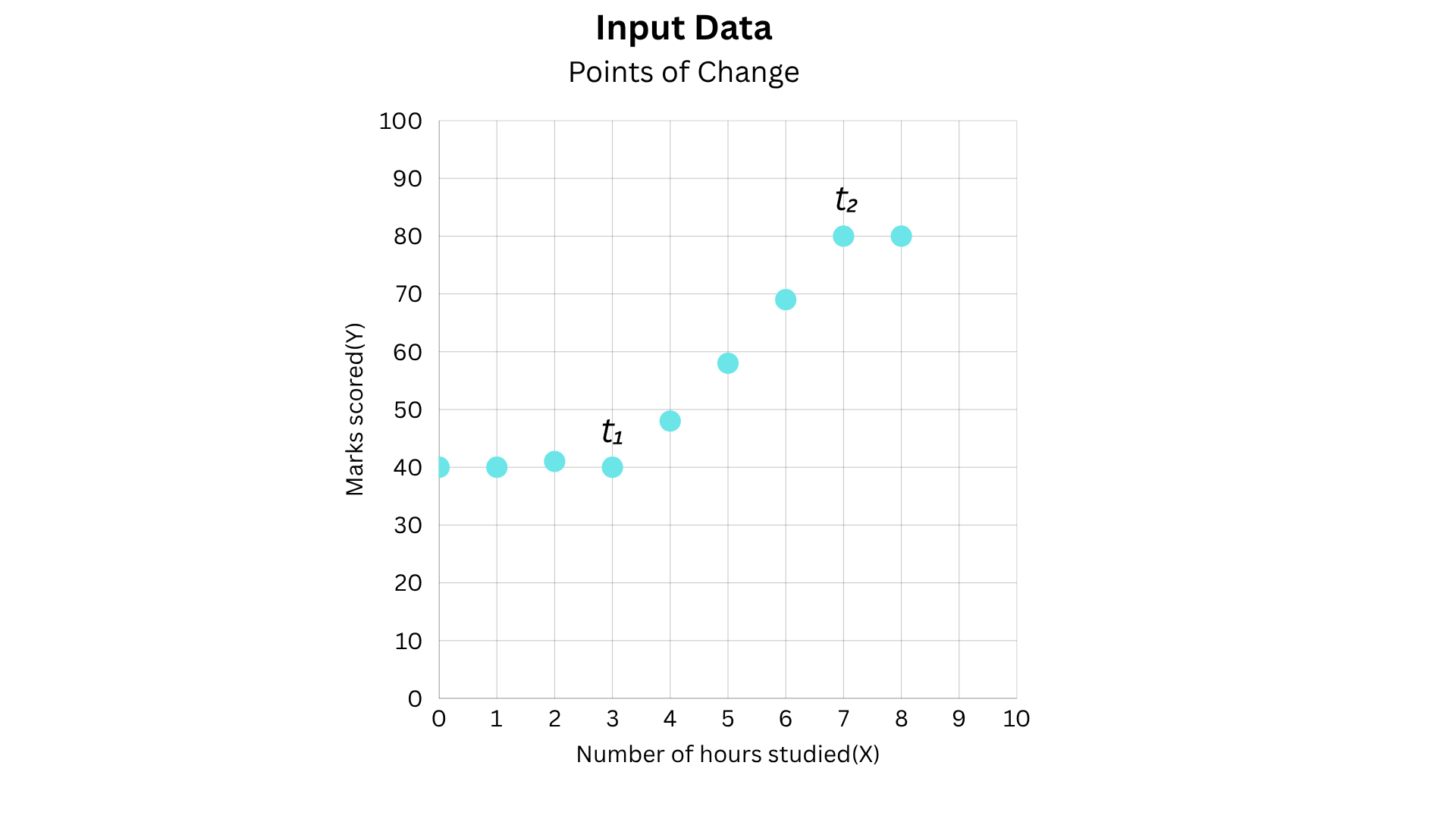
1. Low Study Hours ($x < t_1$): Marks remain relatively constant at a baseline level.
2. Moderate Study Hours ($t_1 le x < t_2$): Marks increase proportionally with study time.
3. High Study Hours ($x ge t_2$): Marks flatten out due to cognitive limits or testing maximums.

By applying separate equations for each distinct range, she entered the realm of piecewise linear functions—functions constructed from multiple linear segments stitched together. While each individual segment is straight, the aggregate curve is fundamentally non-linear.

---

3. Supporting Data: Mathematical Frameworks of Non-Linearity

To transition from conceptual math to machine learning architecture, data scientists utilize specific mathematical functions to inject non-linearity into neural networks.

The Rectified Linear Unit (ReLU)

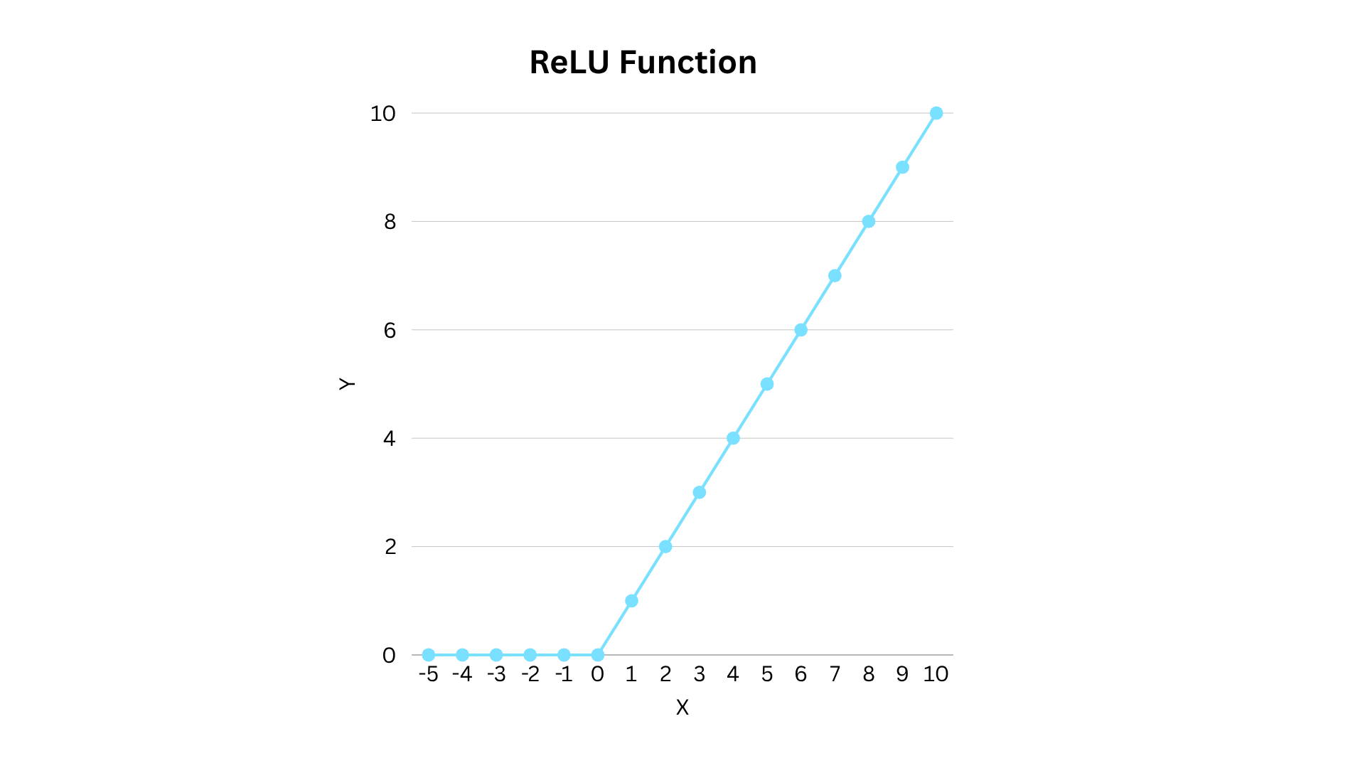
One of the most ubiquitous activation functions in deep learning is the ReLU (Rectified Linear Unit). Mathematically, it is defined as:

$$textReLU(x) = max(0, x)$$

ReLU operates on a simple premise: it passes positive inputs through unchanged while clamping all negative inputs to zero.

• Mechanism: Although individual pieces of the function are linear, the conditional thresholding creates a non-linear global response.
• Utility: It allows a neuron to remain inactive until an input crosses a specific threshold, mimicking biological neurons that only fire when a stimulus surpasses a certain electrical potential.

The Sigmoid Function

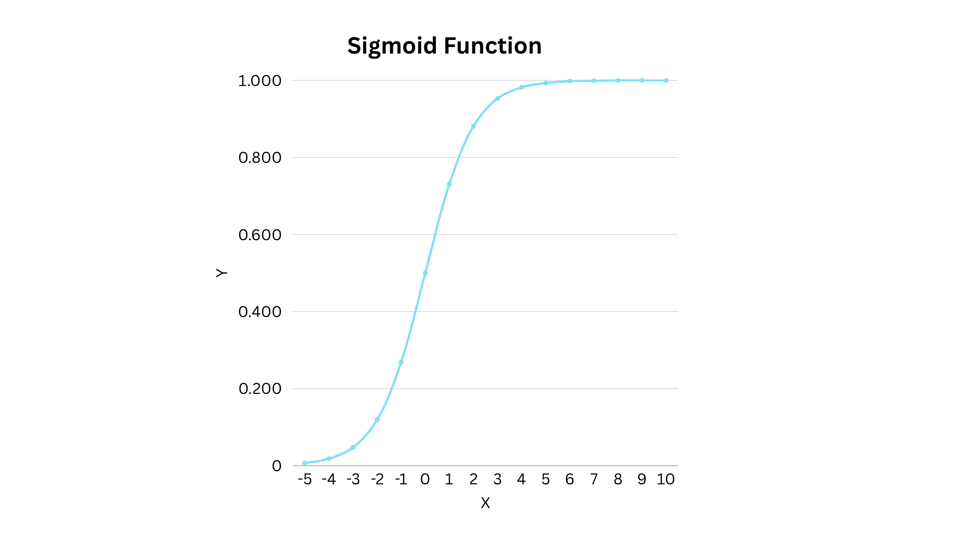
While ReLU excels at unbounded numerical prediction, classification tasks often require outputs bounded between specific probabilities (e.g., passing or failing an exam). For this, networks utilize the sigmoid function:

$$sigma(x) = frac11 + e^-x$$

• Mechanism: The sigmoid function maps any real-valued number into an S-shaped curve bounded strictly between 0 and 1. It rises gradually from zero, accelerates sharply in the middle, and asymptotically approaches unity.
• Utility: The smooth, continuous transition makes it ideal for probability estimation. An output of $0.731$, for instance, can be interpreted as a 73.1% likelihood of a positive outcome.

---

4. Modeling a Deep Neural Network: Practical Execution

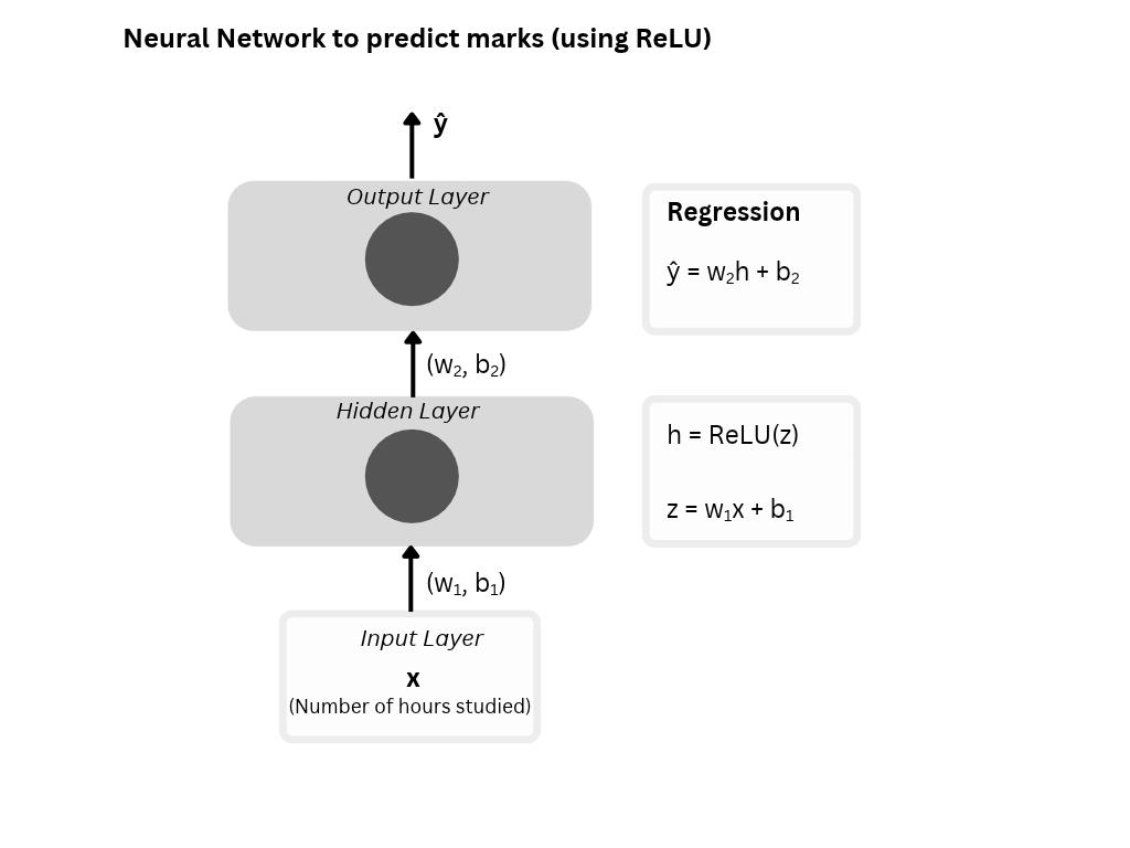
To see how these concepts operate within an artificial neural network, we can examine a simplified, untrained multi-layer perceptron (MLP) mapping study hours to outcomes. In production environments, weights and biases are learned dynamically via backpropagation; here, we set them manually to illustrate computational flow.

Scenario A: Predicting Numerical Marks Using ReLU

1. Setting up the Network:

   

   • Hidden Layer transformation: $z = w_1x + b_1 = x – 3$
   • Activation: $h = textReLU(z)$
   • Output layer: $haty = w_2h + b_2 = 10h + 40$

2. Calculating for a Student Studying 5 Hours ($x = 5$):

   • $z = 5 – 3 = 2$
   • $h = max(0, 2) = 2$
   • $haty = 10(2) + 40 = 60$ marks.

The network predicts 60 marks, closely approximating the actual dataset value of 58. Crucially, because of the ReLU activation, the network avoids the trap of a perpetual straight-line increase, demonstrating how hidden layers capture real-world inflection points.

Scenario B: Predicting Pass/Fail Using ReLU and Sigmoid

Next, the network evaluates whether a student passes or fails, establishing a threshold where a score below 50 constitutes a failure.

1. Setting up the Network:

   • Hidden transformation: $z_1 = x – 4$
   • Hidden activation: $h = textReLU(z_1)$
   • Output transformation: $z_2 = 2h – 1$
   • Probability estimation: $p = sigma(z_2)$

2. Evaluating a Student Studying 3 Hours ($x = 3$):

   • $z_1 = 3 – 4 = -1$
   • $h = max(0, -1) = 0$
   • $z_2 = 2(0) – 1 = -1$
   • $p = frac11 + e^-(-1) approx 0.269$

Since $0.269 < 0.5$, the network classifies the result as Fail.

3. Evaluating a Student Studying 5 Hours ($x = 5$):
   • $z_1 = 5 – 4 = 1$
   • $h = max(0, 1) = 1$
   • $z_2 = 2(1) – 1 = 1$
   • $p = frac11 + e^-1 approx 0.731$

Since $0.731 > 0.5$, the network classifies the result as Pass.

Study Hours	Actual Marks	Actual Result	Predicted Score	Predicted Result
0	40	Fail	0.269	Fail
2	41	Fail	0.269	Fail
4	48	Fail	0.269	Fail
5	58	Pass	0.731	Pass
7	80	Pass	0.993	Pass
8	80	Pass	0.999	Pass

Through this dual-layer approach, the combination of ReLU (for internal feature transformation) and sigmoid (for probabilistic output scaling) enables the network to make accurate, threshold-based classifications.

---

5. Implications for Artificial Intelligence and Future Research

The transition from linear models to non-linear neural networks is not merely an academic exercise; it is the foundational pillar of modern deep learning.

• Universal Approximation: Mathematical theorems (such as the Universal Approximation Theorem) prove that a feedforward neural network with a single hidden layer containing non-linear activation functions can approximate any continuous function to any desired degree of accuracy. Without non-linearity, stacking ten linear layers is mathematically equivalent to stacking a single linear layer, rendering deep architectures useless.
• Handling High-Dimensional Complexity: In advanced domains such as computer vision, natural language processing, and generative AI, data features interact in profoundly non-linear ways. Recognizing edges in images, interpreting semantic context in language, or generating coherent synthetic media requires models that can bend, twist, and partition high-dimensional space. Non-linear activation functions provide the geometric flexibility required to carve decision boundaries through complex data manifolds.

Conclusion

Straight lines are powerful tools for simple, consistent phenomena, but they break down when confronted with the nuances of the physical and digital worlds. By integrating non-linear activation functions like ReLU and sigmoid architectures, neural networks transcend the constraints of elementary geometry. They gain the ability to learn, adapt, and accurately model the complex, shifting patterns that define human experience and modern artificial intelligence.